Hyperbolic Intuition II (Lorentz Model)#
This tutorial has the goal to better understand the Lorentz model, and its accompanying manifold which is often referred to as the Hyperboloid. In contrast to the Poincaré Ball discussed in the previous tutorial, the Hyperboloid does not have a border where the distance between the points reaches infinity and some other nice mathematical properties that are adequately discussed in the literature. The most striking point about the Lorentz Model is that it needs an additional dimension compared to the euclidean space. I am not an expert in this, but the current model of space-time is a Lorentz Model where the additional 0th dimension in addition to our three euclidean dimensions of space is time. Thus, you might see this 0th dimension referred to as time in some of the implementations. For our case, lets start with a simple point cloud in 2-dimensional euclidean space
def map_colors(values):
    import matplotlib as mpl

    cmap = mpl.colormaps["viridis"]

    values = values.pow(2).sum(dim=1).sqrt()

    values = values - values.min()

    values = values / values.max()

    return cmap(values)
import torch
import matplotlib.pyplot as plt
fig, ax = plt.subplots(figsize=(5,5))
x = torch.rand(1000,2)
x = x - x.mean()
colors = map_colors(x)
ax.scatter(x[:, 0], x[:, 1], s=1, c=colors)
<matplotlib.collections.PathCollection at 0x7f908bced180>
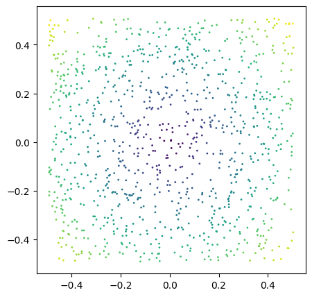
To map these onto the Hyperboloid, we need to add a third dimension at position 0 which only contains zeros:
from torch_hyperbolic.manifolds import Hyperboloid
import math

curvature = 1
point_indices = [1, 14]

ball = Hyperboloid()

colors = map_colors(x)

x_0 = torch.zeros((x.shape[0],)).unsqueeze(-1)

x_0 = torch.cat((x_0, x), dim=-1)

x_balled = ball.proj(ball.expmap0(x_0, c=curvature), c=curvature)
x_back_euclidean = ball.proj_tan0(ball.logmap0(x_balled, c=curvature), c=curvature)
fig = plt.figure(figsize=plt.figaspect(0.33))

for i, (values, title) in enumerate(zip([x_0, x_balled, x_back_euclidean], ["Euclidean", "Hyperbolic", "Back to Euclidean"])):
    ax = fig.add_subplot(1,3,i+1, projection='3d')
    ax.scatter(values[:, 1], values[:, 2], values[:, 0], s=1, c=colors)
    ax.set_title(title)

plt.tight_layout()

We see that, in contrast to the Poincaré Ball, this manifold looks like a blanket that is being pulled up by its corners. We can chosse different values for curvature and track how the shape of the manifold and the distance between two given points are affected by it:
curvatures = [None, 1, 5, 10]

#point_indices = x.pow(2).sum(dim=-1).argsort()[0:2].tolist()
fig = plt.figure(figsize=plt.figaspect(0.25))
for i, curvature in enumerate(curvatures):
    ax = fig.add_subplot(1,4,i+1, projection='3d')
    if curvature is None:
        ax.scatter(x_0[:, 1], x_0[:, 2], x_0[:, 0], s=1, c=colors)
        ax.scatter(x_0[point_indices, 1], x_0[point_indices, 2], x_0[point_indices, 0], s=10, c="r")
        distance_x = x_0[point_indices[0], 0] - x_0[point_indices[1], 0]
        distance_y = x_0[point_indices[0], 1] - x_0[point_indices[1], 1]
        distance = math.sqrt((distance_x ** 2) + (distance_y ** 2))
        ax.set_title("Input Space\nd={:.2}".format(distance))
    else:
        values = ball.proj(ball.expmap0(x_0, c=curvature), c=curvature)
        ax.scatter(values[:, 1], values[:, 2], values[:, 0], s=1, c=colors)
        ax.scatter(values[point_indices, 1], values[point_indices, 2], values[point_indices, 0], s=10, c="r")
        distance = math.sqrt(ball.sqdist(values[point_indices[0],:], values[point_indices[1], :], c=curvature))
        ax.set_title("Curvature {}\nd={}".format(curvature, round(distance, 3)))
    ax.set_xlim((-1,1))
    ax.set_ylim((-1,1))
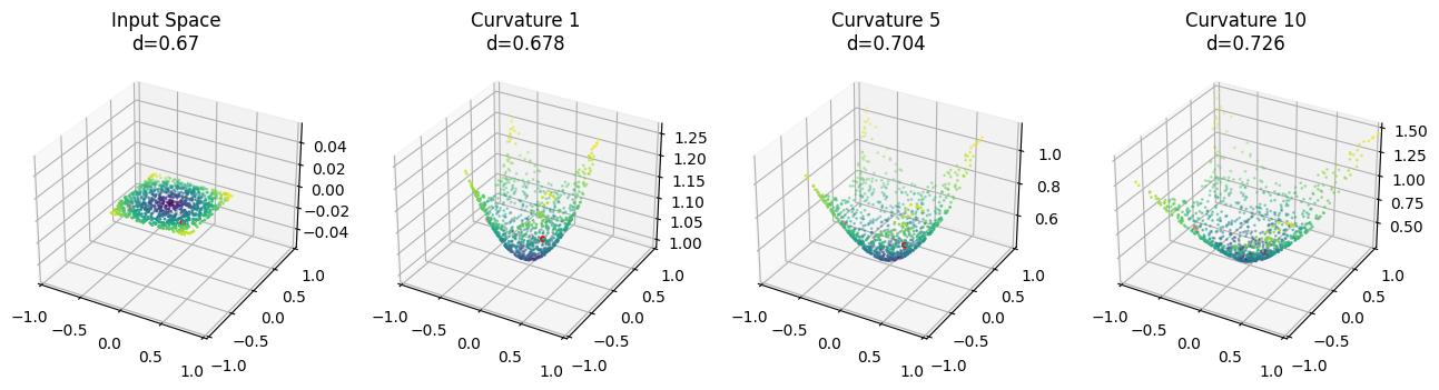
Now, we can choose two values which are closer to the center and we’ll see that the curvature of the manifold has less of an impact on their distance, as distance increases exponentially the further we go away from the center:
curvatures = [None, 1, 5, 10]

point_indices = x.pow(2).sum(dim=-1).argsort()[0:2].tolist()

fig = plt.figure(figsize=plt.figaspect(0.25))

for i, curvature in enumerate(curvatures):
    ax = fig.add_subplot(1,4,i+1, projection='3d')
    if curvature is None:
        ax.scatter(x_0[:, 1], x_0[:, 2], x_0[:, 0], s=1, c=colors)
        ax.scatter(x_0[point_indices, 1], x_0[point_indices, 2], x_0[point_indices, 0], s=10, c="r")
        distance_x = x[point_indices[0], 0] - x[point_indices[1], 0]
        distance_y = x[point_indices[0], 1] - x[point_indices[1], 1]
        distance = math.sqrt((distance_x ** 2) + (distance_y ** 2))
        ax.set_title("Input Space\nd={:.5}".format(distance))
    else:
        x_balled = ball.proj(ball.expmap0(x_0, c=curvature), c=curvature)
        ax.scatter(x_balled[:, 1], x_balled[:, 2], x_balled[:, 0], s=1, c=colors)
        ax.scatter(x_balled[point_indices, 1], x_balled[point_indices, 2], x_balled[point_indices, 0], s=10, c="r")
        distance = math.sqrt(ball.sqdist(x_balled[point_indices[0],:], x_balled[point_indices[1], :], c=curvature))
        ax.set_title("Curvature {}\nd={}".format(curvature, round(distance, 5)))
        ax.set_ylim((-1,1))
        ax.set_xlim((-1,1))

Linear Transformations#
Now, let’s see how linear transformations such as matrix multiplication affects the point cloud and the manifold:
parameters = torch.rand((3,3)).double()
point_indices = [1, 14]


def plot_transformations(x, parameters, point_indices):

        curvature = 10

        a = x_0.double()

        b = torch.mm(a, parameters)

        b[:, 0] = 0

        c = ball.proj(ball.expmap0(b, c=curvature), c=curvature)

        d = ball.proj(ball.expmap0(a, c=curvature), c=curvature)

        e = ball.proj(ball.mobius_matvec(parameters, d, c=curvature), c=curvature)

        f = ball.logmap0(e, c = curvature)

        f[:, 0] = 0

        titles = ["a. Euclidean Input\n$d={}$",
                "b. Euclidean Transformation\n$d={}$",
                "c. Euclidean Transf. into Hyperbolic\n$d={}$",
                "d. Hyperbolic Input\n$d={}$",
                "e. Möbius Matvec Transformation\n$d={}$",
                "f.Möbius Transf. into Euclidean\n$d={}$"]

        fig = plt.figure(figsize=plt.figaspect(0.4))

        for i, values in enumerate([a, b, c, d, e, f]):
                ax = fig.add_subplot(2,3,i+1, projection='3d')
                ax.scatter(values[:, 1], values[:, 2], values[:, 0], s=1 , c=colors)
                ax.scatter(values[point_indices, 1], values[point_indices, 2], values[point_indices, 0], s=10, c="r")
                if i < 2 or i == 5:
                        distance_x = values[point_indices[0], 1] - values[point_indices[1], 1]
                        distance_y = values[point_indices[0], 2] - values[point_indices[1], 2]
                        distance = math.sqrt((distance_x ** 2) + (distance_y ** 2))
                else:
                        distance = math.sqrt(ball.sqdist(values[point_indices[0],:], values[point_indices[1], :], c=curvature))
                ax.set_title(titles[i].format(round(distance,2)))

        plt.tight_layout()

plot_transformations(x, parameters, point_indices)

Here we see our input in euclidean space (a), which is transformed by a matrix multiplication (b). We also see the input transformed into the hyperbolic space (d), tand then transformed (e). We can see that the matrix multiplication affects the point cloud similarly in both spaces, and that the procedure is equivalent by comparing b with d and e with c. In fact, the Mobius Matrix-Vector multiplication implemented in the Hyperboloid simply maps the input from the hyperbolic to the euclidean space, does matrix multiplication there and maps it back again. Just like the Poincaré Ball, very large values are offset to a fixed distance to prevent the occurence of infinite or undefined values:
plot_transformations(x, parameters*100, point_indices)

Bias Addition II#
Another normal building block of neural networks are bias additions. We can to the bias addition in the euclidean space and then project the values into the hyperbolic space or do it directly in hyperbolic space via the Möbius addition:
from torch_hyperbolic.manifolds import Hyperboloid

ball = Hyperboloid()
parameters = torch.rand(3,).double()
point_indices = [1, 14]

def plot_addition(x, parameters, point_indices):

        curvature = 10

        a = x.double()

        parameters = ball.proj_tan0(parameters.squeeze().view(1, -1), c=curvature)

        b = a + parameters

        c = ball.proj(ball.expmap0(b, c=curvature), c=curvature)

        d = ball.proj(ball.expmap0(a, c=curvature), c=curvature)

        hyperbolic_bias = ball.proj(ball.expmap0(parameters, c=curvature),c=curvature)

        e = ball.proj(ball.mobius_add(d, hyperbolic_bias, c=curvature), c=curvature)

        f = ball.logmap0(e, c = curvature)

        f = ball.proj_tan0(f, c = curvature)

        fig = plt.figure(figsize=plt.figaspect(0.47))

        titles = ["a. Euclidean Input\n$d={}$",
                "b. Euclidean Addition\n$d={}$",
                "c. Euclidean Add. into Hyperbolic\n$d={}$",
                "d. Hyperbolic Input\n$d={}$",
                "e. Möbius Addition\n$d={}$",
                "f. Möbius Add. into Euclidean\n$d={}$"]

        for i, values in enumerate([a, b, c, d, e, f]):
                ax = fig.add_subplot(2,3,i+1, projection='3d')
                ax.scatter(values[:, 1], values[:, 2], values[:, 0], s=1, c=colors)
                ax.scatter(values[point_indices, 1], values[point_indices, 2],  values[point_indices, 0],  s=3, c="r")
                if i < 2 or i == 5:
                        distance_x = values[point_indices[0], 0] - values[point_indices[1], 0]
                        distance_y = values[point_indices[0], 1] - values[point_indices[1], 1]
                        distance = math.sqrt((distance_x ** 2) + (distance_y ** 2))
                else:
                        distance = math.sqrt(ball.sqdist(values[point_indices[0],:], values[point_indices[1], :], c=curvature))
                ax.set_title(titles[i].format(round(distance,2)))

        plt.tight_layout()

plot_addition(x_0, parameters, point_indices)

However, when we compare b with f and c with e, we can see that the two procedures are not equivalent, although the literature suggests it. although e looks comparable to c, the distance between the two selected points and the absolute values are different. It is, however, also possible to use the hyperbolic layers implemented in pytorch_geometric withou bias addition.