Hyperbolic Intuition#
This guide is about how hyperbolic features and transformations look like, so you and I can gain an intuition about what happens (and what can go wrong)
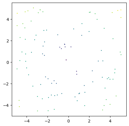
First, lets initialize an array of random 2-dimensional values:
import torch
import matplotlib.pyplot as plt

def map_colors(values):
    import matplotlib as mpl

    cmap = mpl.colormaps["viridis"]

    values = values.pow(2).sum(dim=1).sqrt()

    values = values - values.min()

    values = values / values.max()

    return cmap(values)

fig, ax = plt.subplots(figsize=(5,5))
x = torch.rand(100,2) * 10
x = x - x.mean()

colors = map_colors(x)
ax.scatter(x[:, 0], x[:, 1], s=1, c=colors)
<matplotlib.collections.PathCollection at 0x7ff431240fa0>
In our next step, we will initialize a Poincaré Ball Manifold and project the values on that manifold by using the exponentional map at point 0 and back into the euclidean space. We will also pick out two points so we can track how they move. And add a grey circle at the edge of the Poincaré Disk.
from torch_hyperbolic.manifolds import PoincareBall
import math

curvature = 1
point_indices = [1, 14]

ball = PoincareBall()
x_balled = ball.expmap0(x, c=curvature)
x_back_euclidean = ball.logmap0(x_balled, c=curvature)
fig, axes = plt.subplots(ncols=3, nrows=1, figsize=(15,5))

for ax, values, title in zip(axes, [x, x_balled, x_back_euclidean], ["Euclidean", "Hyperbolic", "Back to Euclidean"]):
    ax.scatter(values[:, 0], values[:, 1], s=1, c=colors)
    ax.scatter(values[point_indices, 0], values[point_indices, 1], s=3, c="r")
    radius = 1/math.sqrt(curvature)
    circle2 = plt.Circle((0, 0), radius, color='lightgray', fill=False)
    ax.add_patch(circle2)
    ax.set_title(title)

as you can see, our values are now on the 2-dimensional Poincaré Ball Manifold, i.e. the Poincaré Disk. The disk has a radius of 1/sqrt(c) where c is the curvature of the manifold. We can use different curvatures to see that the transformation of our input values will yield different results:
ball = PoincareBall()
curvatures = [1, 3, 5]

fig, axes = plt.subplots(ncols= 3, nrows=1, figsize=(15,5))

for ax, curvature in zip(axes, curvatures):
    x_balled = ball.proj(ball.expmap0(x, c=curvature), c=curvature)
    ax.scatter(x_balled[:, 0], x_balled[:, 1], s=1,c=colors)

    radius = 1/math.sqrt(curvature)
    circle2 = plt.Circle((0, 0), radius, color='lightgray', fill=False)
    ax.add_patch(circle2)
    ax.set_title("Curvature {}".format(curvature))
    ax.set_ylim((-1,1))
    ax.set_xlim((-1,1))

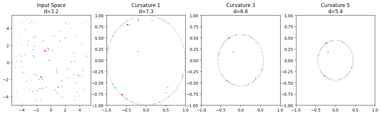
It might look like out values have gotten closer together, especially with higher curvature. However, distance between points increases exponentially the closer we get to the border of the disk, so the actual distance between points is different to what we might intuit. We can showcase this by calculating the distances between two points in the input space and in the three hyperbolic spaces:
ball = PoincareBall()
curvatures = [None, 1, 3, 5]

point_indices = [1, 14]

fig, axes = plt.subplots(ncols= 4, nrows=1, figsize=(16,4))

for ax, curvature in zip(axes, curvatures):
    if curvature is None:
        ax.scatter(x[:, 0], x[:, 1], s=1, c=colors)
        ax.scatter(x[point_indices, 0], x[point_indices, 1], s=5, c="r")
        distance_x = x[point_indices[0], 0] - x[point_indices[1], 0]
        distance_y = x[point_indices[0], 1] - x[point_indices[1], 1]
        distance = math.sqrt((distance_x ** 2) + (distance_y ** 2))
        ax.set_title("Input Space\nd={:.2}".format(distance))
    else:
        x_balled = ball.proj(ball.expmap0(x, c=curvature), c=curvature)
        ax.scatter(x_balled[:, 0], x_balled[:, 1], s=1, c=colors)
        ax.scatter(x_balled[point_indices, 0], x_balled[point_indices, 1], s=5, c="r")
        distance = math.sqrt(ball.sqdist(x_balled[point_indices[0],:], x_balled[point_indices[1], :], c=curvature))
        radius = 1/math.sqrt(curvature)
        circle2 = plt.Circle((0, 0), radius, color='lightgray', fill=False)
        ax.add_patch(circle2)
        ax.set_title("Curvature {}\nd={}".format(curvature, round(distance, 1)))
        ax.set_ylim((-1,1))
        ax.set_xlim((-1,1))
Now, lets repeat this process with two points that are closer to the origin:
ball = PoincareBall()
curvatures = [None, 1, 3, 5]

point_indices = x.pow(2).sum(dim=-1).argsort()[0:2].tolist()

fig, axes = plt.subplots(ncols= 4, nrows=1, figsize=(16,4))

for ax, curvature in zip(axes, curvatures):
    if curvature is None:
        ax.scatter(x[:, 0], x[:, 1], s=1, c=colors)
        ax.scatter(x[point_indices, 0], x[point_indices, 1], s=5, c="r")
        distance_x = x[point_indices[0], 0] - x[point_indices[1], 0]
        distance_y = x[point_indices[0], 1] - x[point_indices[1], 1]
        distance = math.sqrt((distance_x ** 2) + (distance_y ** 2))
        ax.set_title("Input Space\nd={:.2}".format(distance))
    else:
        x_balled = ball.proj(ball.expmap0(x, c=curvature), c=curvature)
        ax.scatter(x_balled[:, 0], x_balled[:, 1], c=colors, s=1)
        ax.scatter(x_balled[point_indices, 0], x_balled[point_indices, 1], s=5, c="r")
        distance = math.sqrt(ball.sqdist(x_balled[point_indices[0],:], x_balled[point_indices[1], :], c=curvature))
        radius = 1/math.sqrt(curvature)
        circle2 = plt.Circle((0, 0), radius, color='lightgray', fill=False)
        ax.add_patch(circle2)
        ax.set_title("Curvature {}\nd={}".format(curvature, round(distance, 3)))
        ax.set_ylim((-1,1))
        ax.set_xlim((-1,1))

Here, we can see that the distances between the three hyperbolic spaces are identical because the points are close to the center.
Transformations#
Next, lets look at how transformations work in hyperbolic space. Linear layers in neural networks are characterized by a multiplication of two matrices and an optional addition of a third. Lets first start with the matrix multiplication:
from torch_hyperbolic.manifolds import PoincareBall
ball = PoincareBall()
parameters = torch.rand((2,2)).double()
point_indices = [1, 14]

def plot_transformations(x, parameters, point_indices):

        a = x.double()

        b = torch.mm(a, parameters)

        curvature = 1

        c = ball.proj(ball.expmap0(b, c=curvature), c=curvature)

        d = ball.proj(ball.expmap0(a, c=curvature), c=curvature)

        e = ball.proj(ball.mobius_matvec(parameters, d, c=curvature), c=curvature)

        f = ball.logmap0(e, c = curvature)

        fig, axes = plt.subplots(ncols= 3, nrows=2, figsize=(16,8))

        titles = ["a. Euclidean Input\n$d={}$",
                "b. Euclidean Transformation\n$d={}$",
                "c. Euclidean Transf. into Hyperbolic\n$d={}$",
                "d. Hyperbolic Input\n$d={}$",
                "e. Möbius Matvec Transformation\n$d={}$",
                "f.Möbius Transf. into Euclidean\n$d={}$"]


        for i, (ax, values) in enumerate(zip(axes.flatten(), [a, b, c, d, e, f])):
                ax.scatter(values[:, 0], values[:, 1], s=1, c=colors)
                ax.scatter(values[point_indices, 0], values[point_indices, 1], s=5, c="r")
                if i < 2 or i == 5:
                        distance_x = values[point_indices[0], 0] - values[point_indices[1], 0]
                        distance_y = values[point_indices[0], 1] - values[point_indices[1], 1]
                        distance = math.sqrt((distance_x ** 2) + (distance_y ** 2))
                else:
                        distance = math.sqrt(ball.sqdist(values[point_indices[0],:], values[point_indices[1], :], c=curvature))
                radius = 1/math.sqrt(curvature)
                circle2 = plt.Circle((0, 0), radius, color='lightgray', fill=False)
                ax.add_patch(circle2)
                ax.set_title(titles[i].format(round(distance,2)))

        plt.tight_layout()

plot_transformations(x, parameters, point_indices)

In these Panels, we can see our euclidean input features (a), and how they are transformed by a matrix multiplication (b). In addition, you see the hyperbolic representation of the input features (d) and how they are transformed using the same parameter matrix but with a Möbius matrix-vector multiplication. Then finally, in c, you see the projection of the euclidean transformed features from b into the hyperbolic space, which should resemble d, and the projection of the hyperbolic transformed features from e into the euclidean space, which should resemble b. In fact, we note that the shapes in b and f or c and e look similar and the distances are similar as well, so these operations are in fact exchangable. However, at extreme points of the manifold which are reserved for very large values, points can get pushed together, which then impacts their values when they are mapped back to the euclidean space, as in frame e:
plot_transformations(x, parameters*5, point_indices)

This is due to the fact that the distance between points very close to
the border are infinite, while points outside of the border are
undefined. As we want to make sure that infinite and undefined values do
not occur in a machine learning pipeline, all points very close or
across the border of the manifold are re-set onto the manifold with a
fixed distance to its border (by the proj() method of the manifold).
This can destroy the initial information of points, but it only is a
problem for very large values.
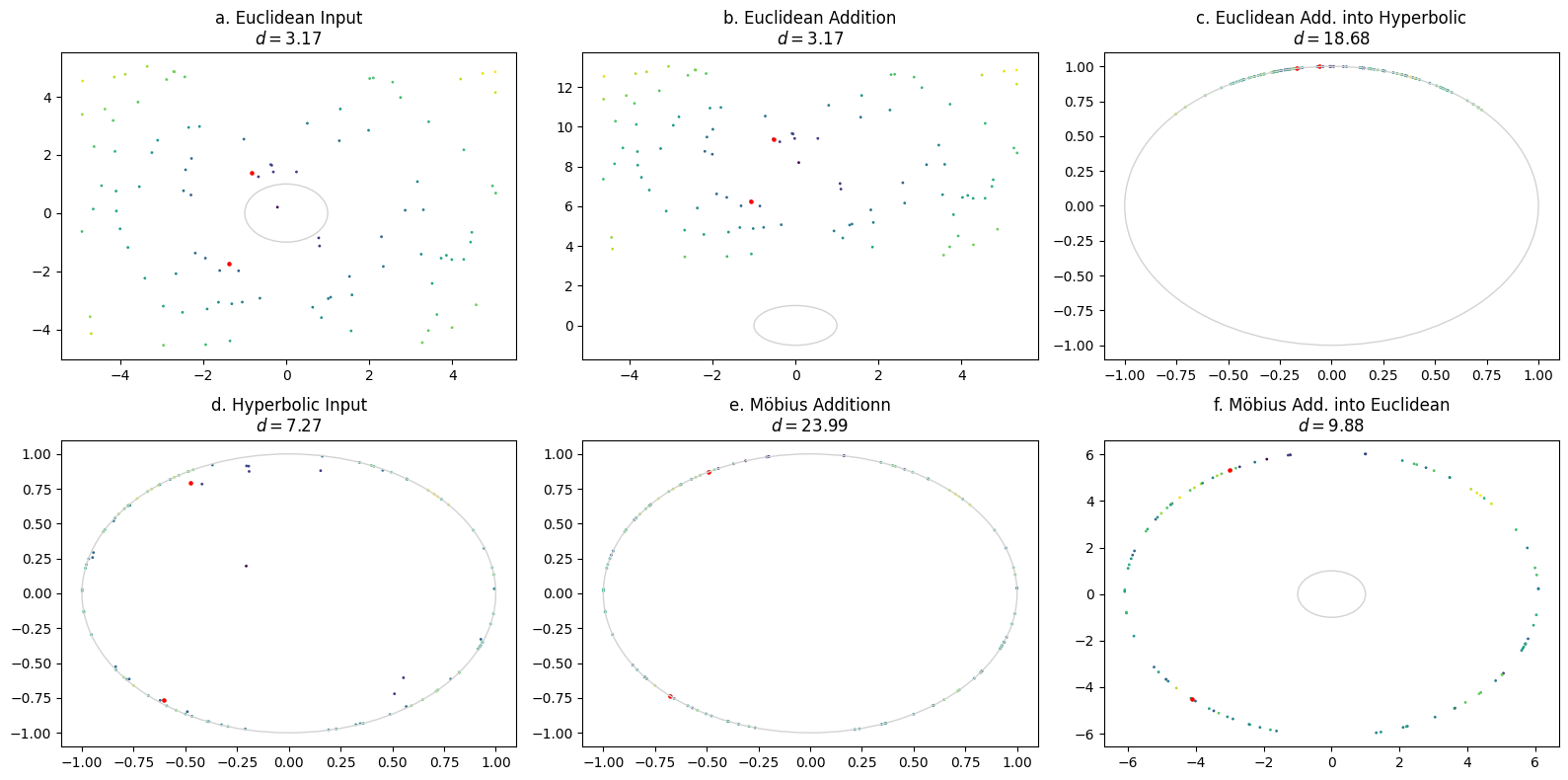
Bias Addition#
from torch_hyperbolic.manifolds import PoincareBall

ball = PoincareBall()
parameters = torch.rand(2,).double()
point_indices = [1, 14]

def plot_addition(x, parameters, point_indices):

        a = x.double()

        b = a + parameters

        curvature = 1

        c = ball.proj(ball.expmap0(b, c=curvature), c=curvature)

        d = ball.proj(ball.expmap0(a, c=curvature), c=curvature)

        hyperbolic_bias = ball.proj(ball.expmap0(parameters, c=curvature),c=curvature)

        e = ball.proj(ball.mobius_add(d, hyperbolic_bias, c=curvature), c=curvature)

        f = ball.logmap0(e, c = curvature)

        fig, axes = plt.subplots(ncols= 3, nrows=2, figsize=(16,8))

        titles = ["a. Euclidean Input\n$d={}$",
                "b. Euclidean Addition\n$d={}$",
                "c. Euclidean Add. into Hyperbolic\n$d={}$",
                "d. Hyperbolic Input\n$d={}$",
                "e. Möbius Additionn\n$d={}$",
                "f. Möbius Add. into Euclidean\n$d={}$"]


        for i, (ax, values) in enumerate(zip(axes.flatten(), [a, b, c, d, e, f])):
                ax.scatter(values[:, 0], values[:, 1], s=1, c=colors)
                ax.scatter(values[point_indices, 0], values[point_indices, 1], s=5, c="r")
                if i < 2 or i == 5:
                        distance_x = values[point_indices[0], 0] - values[point_indices[1], 0]
                        distance_y = values[point_indices[0], 1] - values[point_indices[1], 1]
                        distance = math.sqrt((distance_x ** 2) + (distance_y ** 2))
                else:
                        distance = math.sqrt(ball.sqdist(values[point_indices[0],:], values[point_indices[1], :], c=curvature))
                radius = 1/math.sqrt(curvature)
                circle2 = plt.Circle((0, 0), radius, color='lightgray', fill=False)
                ax.add_patch(circle2)
                ax.set_title(titles[i].format(round(distance,2)))

        plt.tight_layout()

plot_addition(x, parameters, point_indices)

Here, we see the euclidean input again (a), which then gets a bias parameter added (b). In contrast, we also see the input transformed into the hyperbolic space (d), which is then added to the same parameter, which has also been transformed into hyperbolic space (d). The addition between two tensors in hyperbolic space happens via Möbius addition. Panels c and f show the results from b and d, but transformed in the respective other space. This means that b should resemble f and c should resemble e. Again, in some cases, this is true, but if we increase the magnitude of the parameters, as in the next image, this begins to fail:
plot_addition(x, parameters * 10, point_indices)
Just as with the linear transformations, the high values push the points off the manifold, after which they are re-set onto the manifold in a fixed distance to the border to prevent infinite or undefined values. This can destroy the information content of a point, but will only occur for large parameters. If this acts as a kind of inherent regularization remains to be investigated.